Download "Executive Summary/Overview" Chapter
The 2016 Billion-Ton Report: Advancing Domestic Resources for a Thriving Bioeconomy (BT16) evaluates the most recent estimates of potential biomass that could be available for new industrial uses in the future. Volume 1 of this report, presented here, focuses on resource analysis–projecting biomass potentially available at specified prices. Volume 2, targeted for release at the end of 2016, evaluates changes in environmental sustainability indicators associated with select production scenarios in volume 1. Building on previous analyses, BT16 (1) updates the farmgate/roadside analysis using the latest available data and specified enhancements; (2) adds more feedstocks, including algae and specified biomass energy crops; and (3) expands the analysis to include a scenario study to illustrate the cost of transportation to biorefineries under specified logistical assumptions. Here are key summary results and conclusions of BT16 volume 1.
| Feedstock | Million Dry Tons | ||||||||||||||||||||||||||
|---|---|---|---|---|---|---|---|---|---|---|---|---|---|---|---|---|---|---|---|---|---|---|---|---|---|---|---|
| Currently Used Resources | |||||||||||||||||||||||||||
| Forestry Resources Currently Used | |||||||||||||||||||||||||||
| Agricultural Resources Currently Used | |||||||||||||||||||||||||||
| Waste Resources Currently Used | |||||||||||||||||||||||||||
| Total Currently Used | |||||||||||||||||||||||||||
| Potential Resources (For Selected Scenarios) | |||||||||||||||||||||||||||
| Forestry Resources Potential (all timberland)a | |||||||||||||||||||||||||||
| Forestry Resources Potential (no federal timberland)a | |||||||||||||||||||||||||||
| Agricultural Residues Potential | |||||||||||||||||||||||||||
| Energy Crops Potentialb | |||||||||||||||||||||||||||
| Waste Resources Potentialc | |||||||||||||||||||||||||||
| Total (All Timberland)c | |||||||||||||||||||||||||||
| Total (Currently Used + Potential)c | |||||||||||||||||||||||||||
Figure ES.4: County-level map and national bar graph of potential biomass resources (excluding currently used) across the lower 48 states, defaulted to $60 per dry ton per year for the base-case scenario. Feedstock supply is reported by default as a density value, potential county-level supply divided by county land area. Supply quantities in blue are correlated to having a feedstock density of 100 dry tons per square mile or more, which corresponds to the approximate minimum quantity to supply a hypothetical facility at 2,000 dry tons per day.
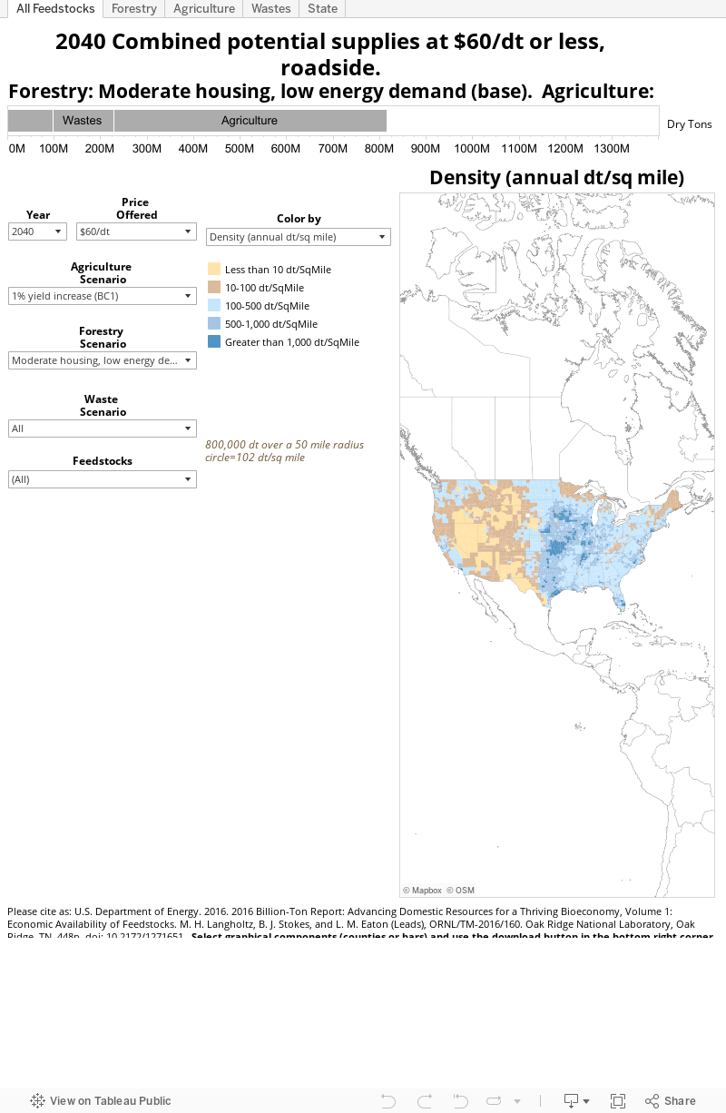
Figure ES.1: County-level map and bar graph of potential primary forestry resources at the county-level for all feedstocks identified in chapter 3, as well as other forest thinnings and other forest residue from chapter 5. Feedstock supply is reported by default as a density value, potential county-level forest landing supply divided by county land area. Supply quantities in blue are correlated to having a feedstock density of 100 dry tons per square mile or more, which corresponds to the approximate minimum quantity to supply a hypothetical facility at 2,000 dry tons per day.
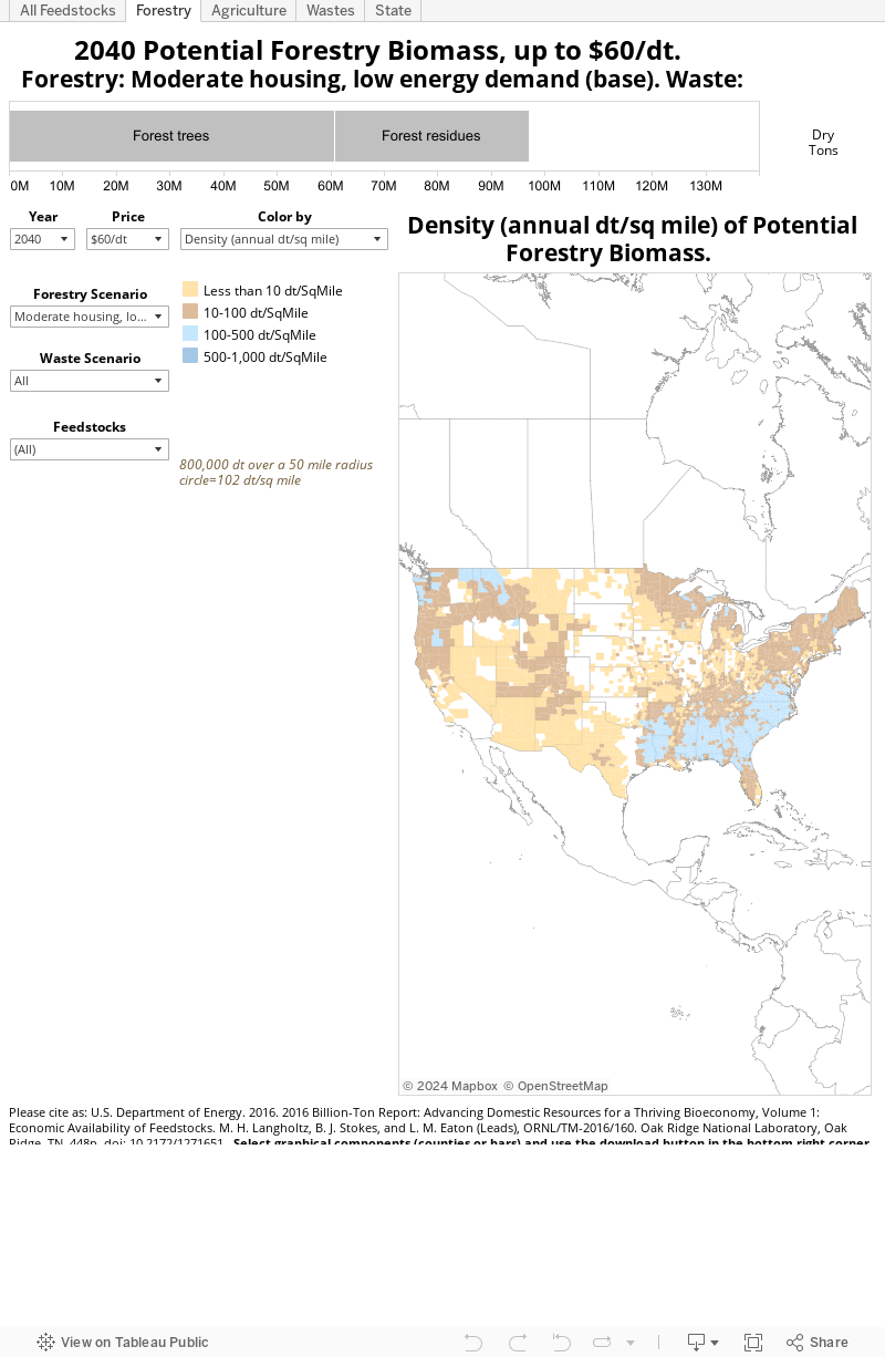
Figure ES.2: County-level map and bar graph of primary agricultural resources at the county-level for all feedstocks identified in chapter 4. Feedstock supply is reported by default as a density value, potential county-level supply at the farmgate divided by county land area. Supply quantities in blue are correlated to having a feedstock density of 100 dry tons per square mile or more, which corresponds to the approximate minimum quantity to supply a hypothetical facility at 2,000 dry tons per day.
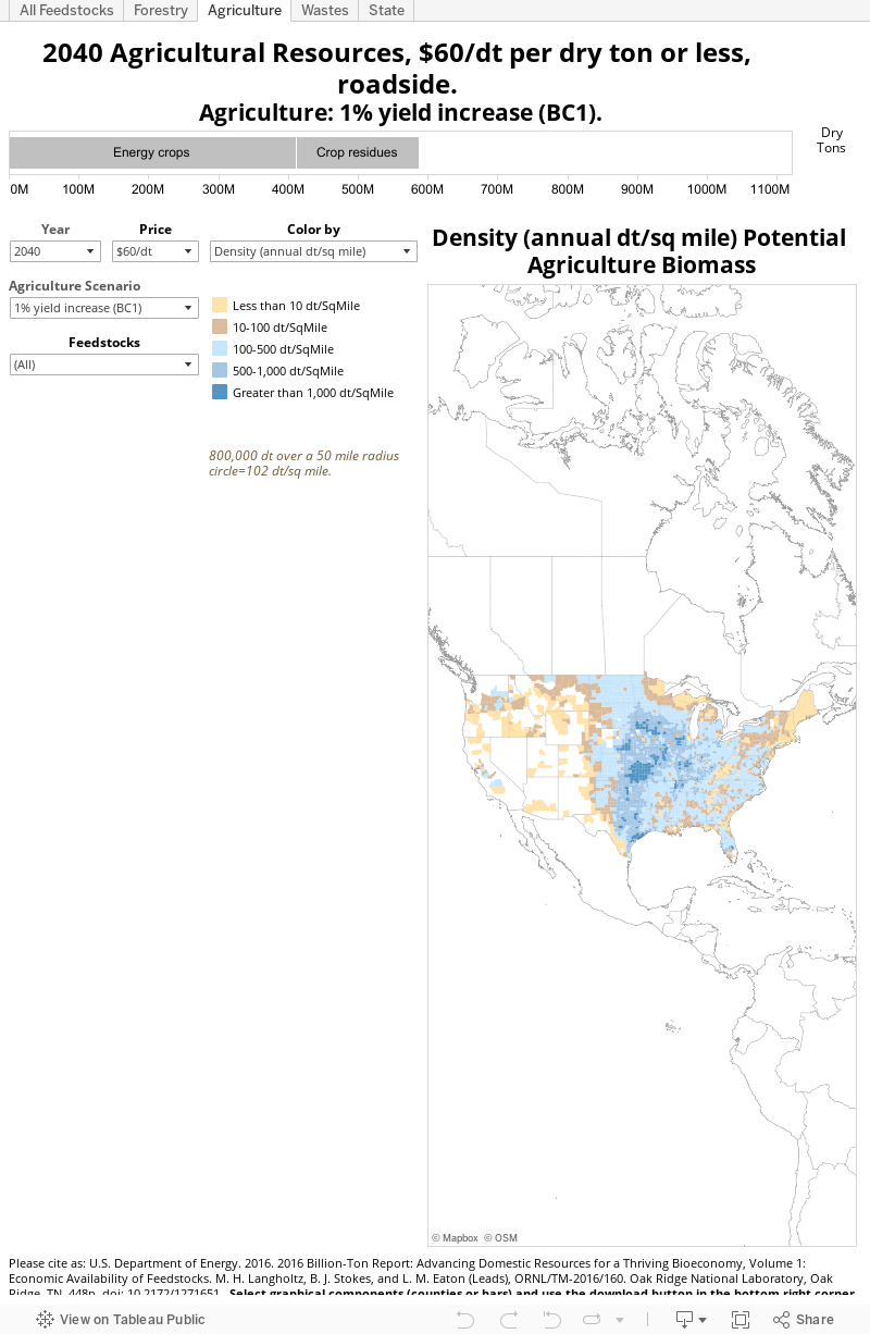
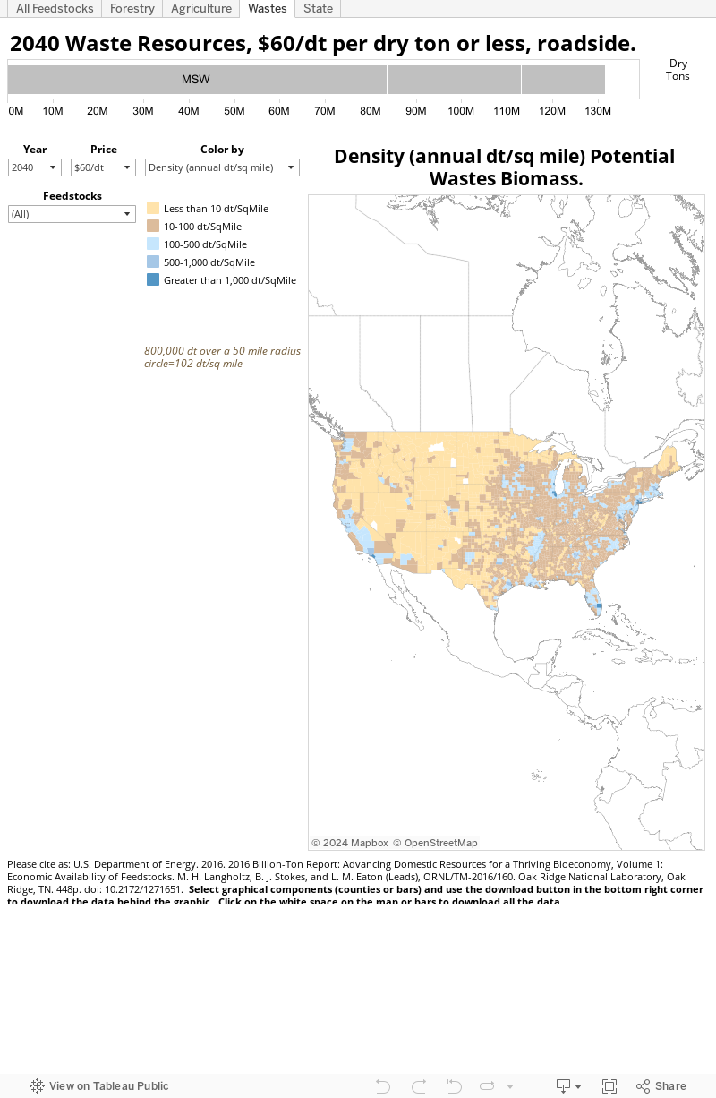
Figure ES.3: County-level map and bar graph of waste resources at the county-level for all feedstocks identified in Chapter 5. Feedstock supply is reported by default as a density value, potential county-level supply at a collection facility divided by county land area. Supply quantities in blue are correlated to having a feedstock density of 100 dry tons per square mile or more, which corresponds to the approximate minimum quantity to supply a hypothetical facility at 2,000 dry tons per day.
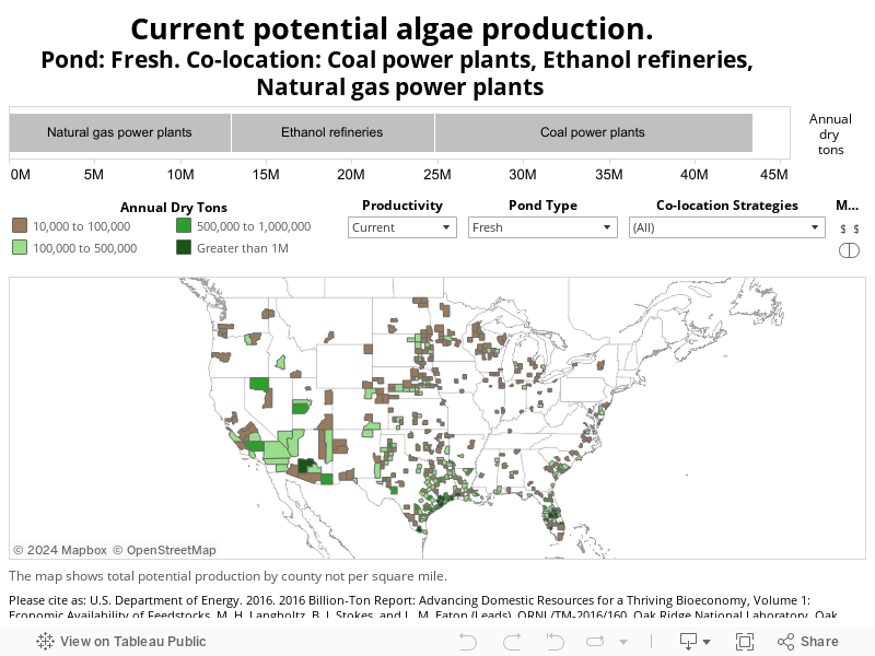
County-level map of algal resources segmented by co-location. Selections for pond type, co-location, present/future, cost range.
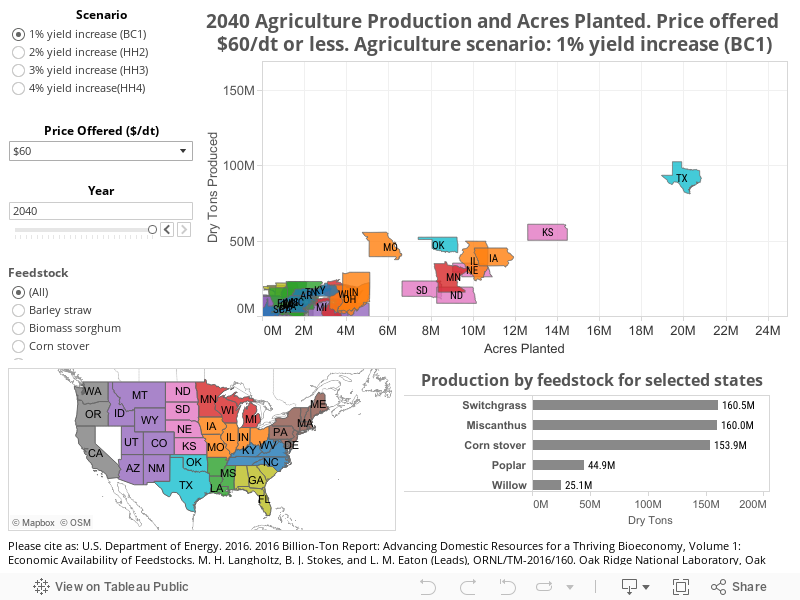
State-level summary plot of feedstock supply and acres planted, bar graph of potential supply, and national map by agricultural production scenario. For detailed state results, click on the state of interest and bar graph repopulates. For detailed crop results, click on the feedstock choice for state-level comparison.
Matrix of year and farmgate price combinations. Select year of interest, biomass price, and scenario for national bar graph and state-level map.
Resource-explicit, stepwise supply curve, including potentially available energy crops, agricultural residues, forestry resources, and waste resources. The marginal supply is represented by stepwise supply and is segmented by biomass type. The weighted average price curve is shown as the black line below the marginal supply boxes. The average price of all total potential supply between $30–$90 is reported at the right tip of the average supply curve. Black line indicates weighted average price.
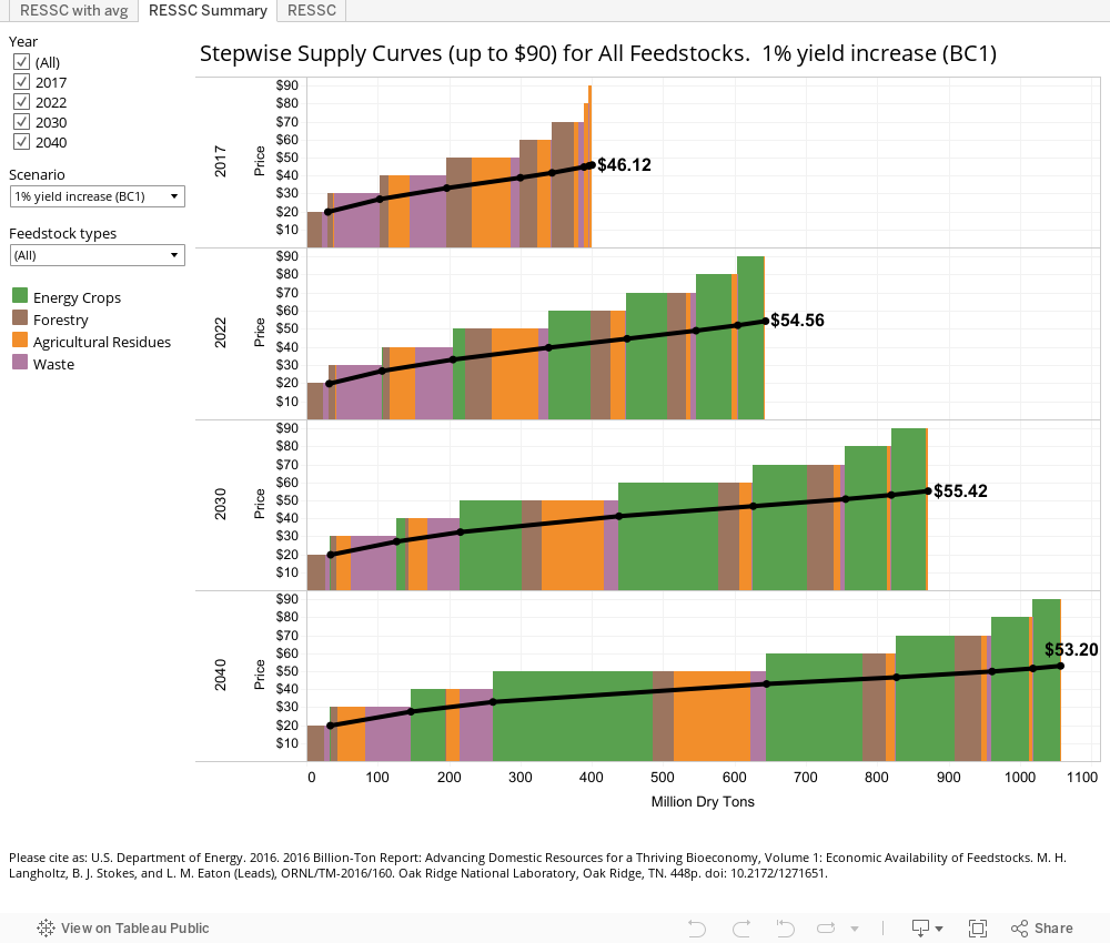
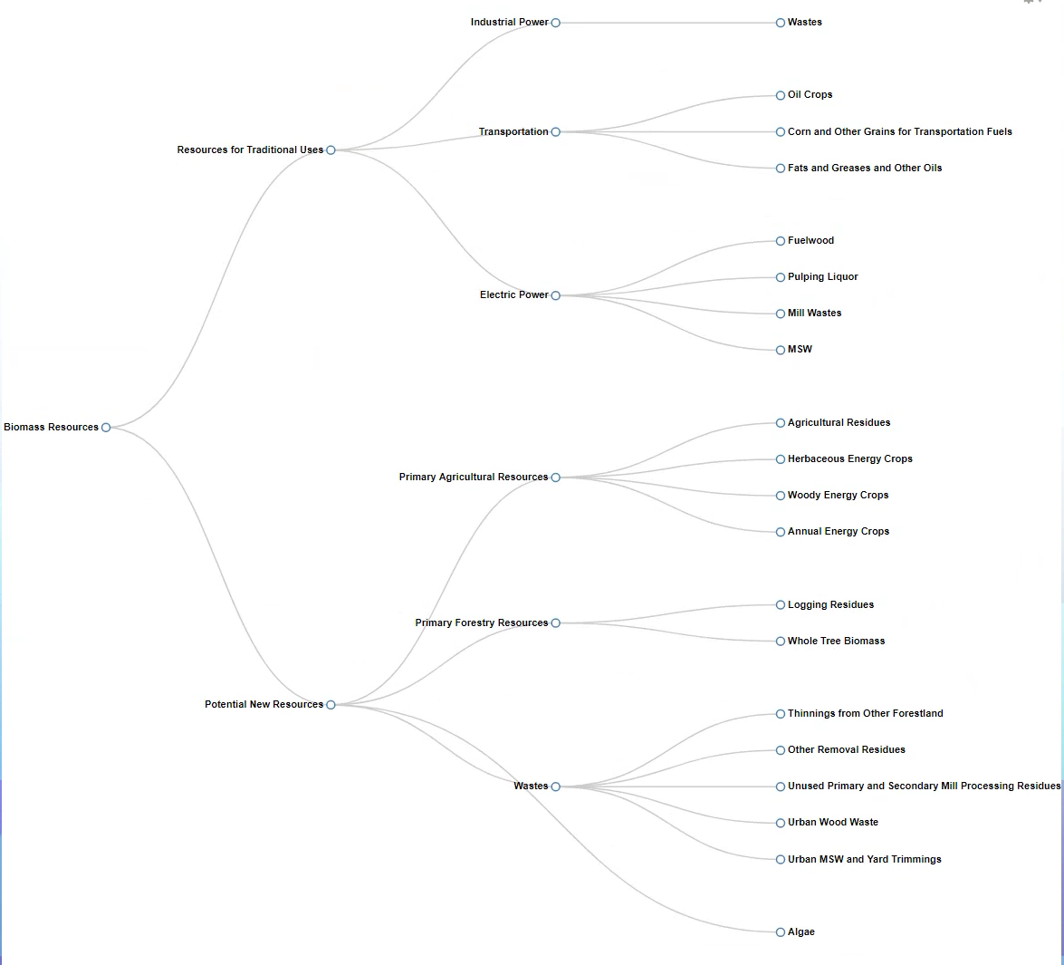
Figure 1.2: Taxonomy of biomass resources identified in BT16. Resources for traditional uses are measured in chapter 2 and sum to 365 million dry tons equivalent per year. Potential new resources are quantified in chapters 3, 4, and 5 and vary depending on biomass price, scenario, and year of interest. Combined, the traditional uses and potential new resources sum to approximately 1.2 billion tons of biomass in 2040 in the base-case scenario.
|
Production
Grower payment, stumpage price, procurement price
|
Harvest
Farmgate price, roadside price
|
Delivery and Processing
Delivered Cost
|
||
|---|---|---|---|---|
| Example Operations: | Site preparation, planning, cultivation, maintenance, profit to landowner | Cut and bale, rake and bale, fell, forward, and chip into van | Load, transport, unload | |
| Format: | In the field or forest, dispersed | Baled or chipped into van roadside | Comminuted to 1/4 inches (conventional) or pelleted (advanced) | |
| Chapters: (3) At the Roadside, Forestland Resources; (4) At the Farmgate, Agricultural Residues and Biomass Crops; (5) Waste Resources; and (7) Microalgae | Chapter (6) To the Biorefinery, Delivered Supplies and Prices | |||
| Chapters (2) Currently Used; (8) Summary, Interpretation, and Looking Forward | ||||
Figure 1.3: Schematic representation of the three major stages of supply chain costing with examples: grower payment, farmgate price, and delivered cost.
Figure ES.5: National marginal supply curve of 2040 biomass resources for agricultural, forestry, and waste resources. Supply curve includes a total marginal biomass supply curve for base-case and high-yield scenarios, with average price curves represented as dashed curves below the marginal supply curves.
